

Disclaimer: Opinions shared in this, and all my posts are mine, and mine alone. They do not reflect the views of my employer(s) and are not investment advice.
In the last few weeks, I’ve been trying to write a post about certain trends I’ve observed in Agentic AI hardware - about CPUs, ISAs, Memory, etc. To do this, I read existing commentary from others to defend my hypothesis, but they all ended up in one of these buckets:
Company marketing highlighting why a specific aspect is more important
Decisions that were made due to the prevailing supply constraints like HBM shortage
A narrow focus on a specific type of agent (typically claude-code style agents)
Since I’m not trying to sell you a chip, I can’t predict the semiconductor supply chain, and I don’t have a favorite agent, I could never complete the post I wanted to write. Instead, I’m taking a step back and starting with a more fundamental question:
How does LLM Inference run locally on your computer?
I’m not going to claim this post will teach you something fundamentally new. In fact, most of what I’m going to talk about is just traditional software execution on a system with a CPU and a GPU. But this post serves as the base camp for some other interesting questions I want to raise in later posts.
What does the software look like?
There are many different ways to launch an LLM inference call. For this post, I’m using a simple Python script that executes the inference using Ollama. This is what the script looks like:
# Import request library to send/recieve HTTP requests
import requests

# Send the LLM Inference call as a HTTP request through Ollama
r = requests.post(
        "http://localhost:11434/api/generate",                           # localhost:11434 indicates that the request should be sent to local Ollama port
    json={                                                               # the model name, prompt, and other settings are passing as the JSON payload
        "model": "qwen3:8b",
        "prompt": "What's more important for Agentic AI - CPU, or GPU?",
        "stream": False,
    },
)

# Print the output of the LLM inference call
print(r.json()["response"])
For this post, this is all you need to know about this script:
The script runs LLM inference using the qwen3:8b model.
The prompt sent to the LLM is “What’s more important for Agentic AI - CPU, or GPU?”
Streaming is disabled - so the final output will be printed only after all output tokens are produced.
What does the hardware look like?
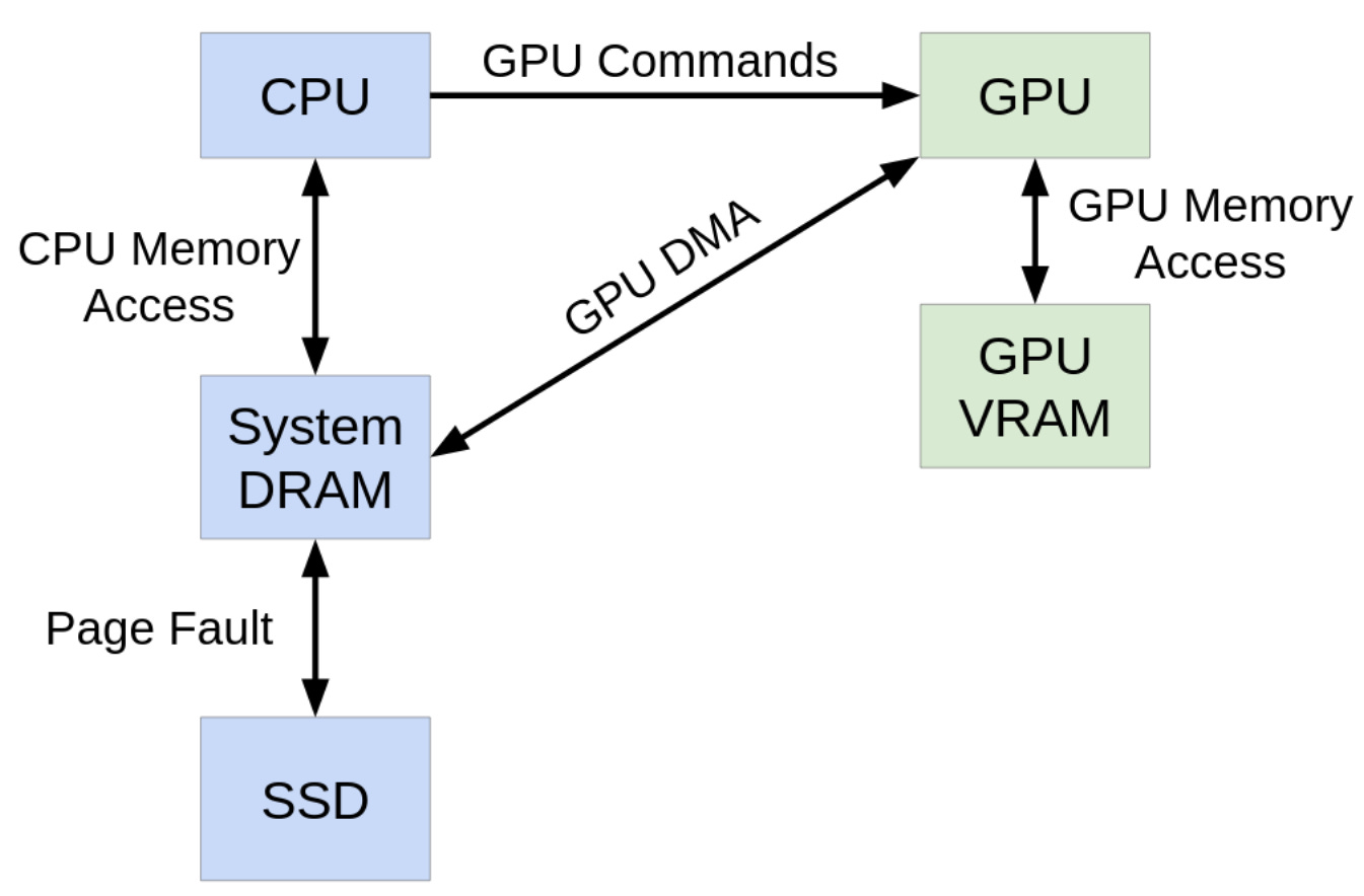
Since the software runs LLM inference locally, (no requests leave the computer where the script was launched) I’m assuming a standard personal computing setup with a host CPU (which runs the Operating System (OS)) and a discrete GPU.
In a system like this, the CPU and GPU typically have separate physical main memories: the CPU accesses System DRAM, while the GPU primarily accesses dedicated Video RAM (VRAM). There is also a large, non-volatile Solid-State Drive (SSD), from which the OS loads data into System DRAM on demand. There are usually more levels in the memory hierarchy, but for simplicity, we will skip these cache effects.
At a high level, this is all you need to know about the CPU-GPU system - I’ll be sharing more details as we walk through the execution.
Is anyone running Local LLMs on their computers?
I expect this question to come up at some point, so I want to get ahead.
You might wonder whether a personal computing hardware architecture like this is relevant in the era of large AI data centers. It’s a fair question, but there are two reasons why I went with local LLM inference on a discrete GPU system:
Datacenter hardware architectures are vendor specific and evolving so quickly, so it’s hard to write a post like this without making a lot of assumptions (which I think would dilute the post.)
I own a computer with a CPU and GPU which I can use to run some profiling for future posts.
But irrespective of the hardware architecture, the fundamental interaction between a CPU running the OS and an accelerator like the GPU will remain largely the same - that’s going to be the key focus of this post.
The shipping analogy
I recently drove past the Port of Los Angeles, the busiest seaport in the US. I knew it was big, but looking out at the large ships and the thousands of containers waiting to be loaded in them left an impression on me. So that’s my excuse to include it as an analogy for this post.

A shipping port is a good analogy for the AI computing landscape because of the heterogeneity. In addition to ships, a port is also closely connected to major freeways, railway lines, and airports - not too different from the different “Processing Units” that we have in the computing world today.
There’s something else that maps well to Agentic AI in particular - the variety of loads handled by a port. The logistics of shipping perishable goods is not the same as automobiles, and is completely different from how a cruise ship would be managed. I think this can be a good mental model to differentiate the requirements of coding agents, versus, say, a robotics pipeline.
Going forward, any references to this analogy will be in quotes to separate it from the rest of the text. Use it to simplify concepts, or to just give yourself a break.
Computer Science 101
I will be using (and have probably already used) a lot of computing terms in this post without properly introducing them, so here’s a quick glossary covering most of them. Skip ahead if you are already familiar with these.
Operating System (OS): It’s the system software that manages everything - from the interaction between CPU, GPU and other hardware resources, to managing permissions to processes and device drivers.
Process: It is a software abstraction created by the OS that provides a virtual address space and resources for running a program. A process contains one or more threads.
CPU Thread: It is an execution context with its own architectural register state and instruction pointer that can be scheduled to run on a CPU core.
CPU Core: Physical CPU hardware that can fetch and execute instructions.
Driver: It is software that allows the OS and applications to interact with a hardware device like the GPU.
GPU Kernel: A function/program executed on the GPU across many parallel threads.
Virtual Address: It is the address used in the software world. The OS and hardware translate it to physical hardware addresses through page tables.
HTTP: A commonly used request/response protocol that allows one application to talk to another. (either within the same system, or through the internet.)
TCP: It is a popular byte-stream protocol used by HTTP connections to transfer data.
JSON: A standard format for serializing structured data like lists, arrays, or dictionaries.
UTF-8: It is a standard encoding that represents unicode text (in JSON) as bytes (binary).
You can think of the OS like the Port Authority which manages port access for different entities.
Each process is like a logistics partner involved in each shipping task - like the company that wants to ship their goods, freight and ship providers, and so on.
Each CPU thread is like a Truck that carries Containers (i.e. data) to the GPU (which is like a Ship), and together they complete the shipping task. (i.e. the LLM inference script.)
LLM Inference Walkthrough
Enough buildup.
Say you have your LLM inference script on a file: llm_inference.py
Let’s look at everything that happens when you launch this command on your shell: python llm_inference.py
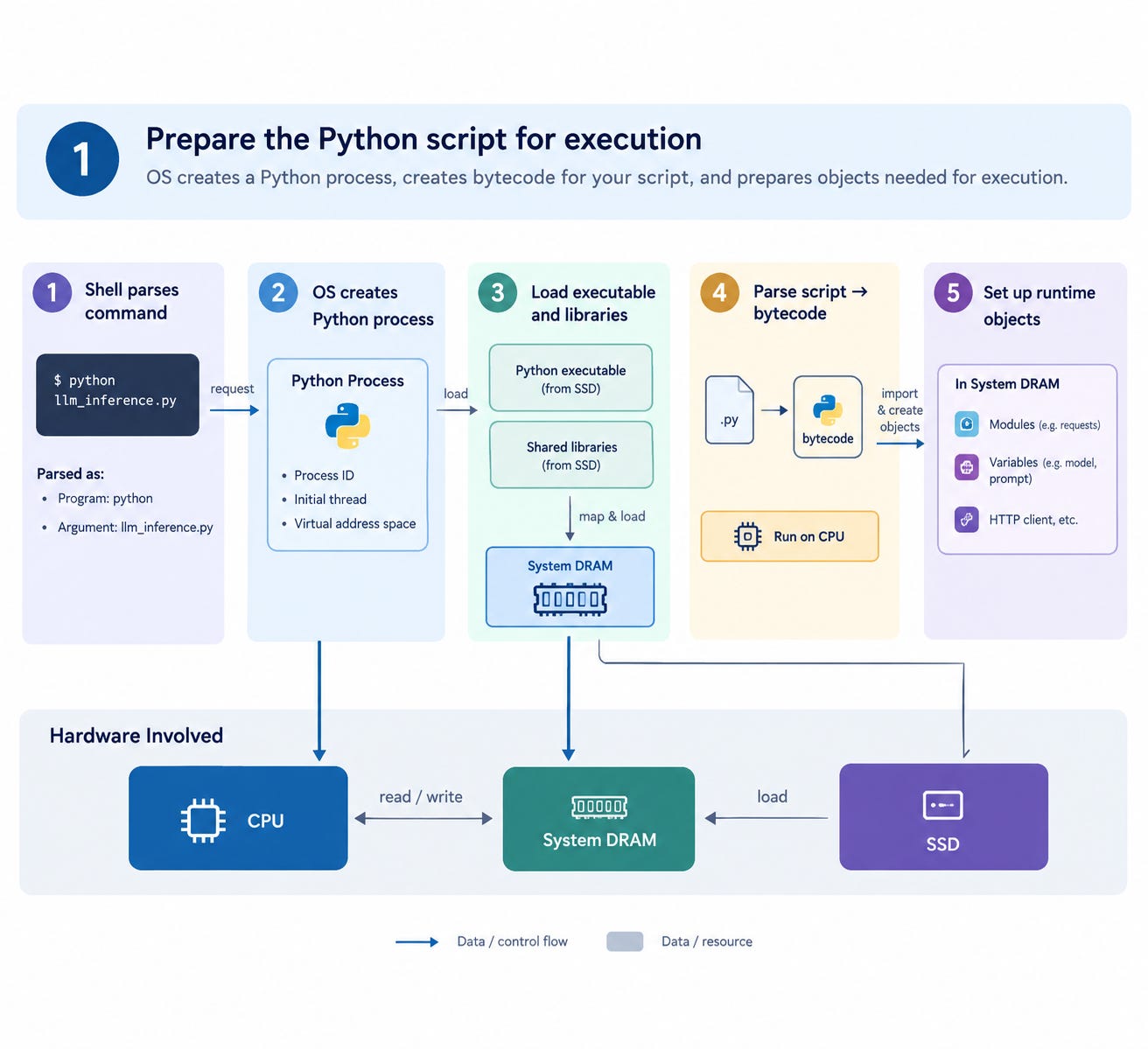
Phase 1: Prepare the Python script for execution
TL;DR: OS creates a Python process, creates bytecode for your script, and prepares objects needed for execution.
Hardware Involved: CPU, System DRAM, and SSD
In this phase, we won’t start physically shipping any goods yet. The Python process is like a company with a shipping request that first gets all the required information and approvals from the port authority (OS) before it can start the shipping task.
Step 1: Shell interprets the command
Your shell (Bash, Powershell, etc.) parses the entered text and interprets it as:
Program to launch: Python
Argument passed: llm_inference.py
Step 2: OS creates a Python process
The shell asks the OS to launch the “Python executable”. (More on this in step 3.) To do this, the OS creates a new Python process. The new Python process is provided with what it needs to execute:
A process ID
An initial thread
Virtual address space that it can access
Whenever we see the Python process “executing” something on the CPU, remember that it is done through this initial thread.
Step 3: OS prepares the Python executable
Once the process is created, the OS maps virtual memory addresses needed for the Python executable to System DRAM locations and loads the pre-compiled Python executable and the required libraries from the CPU SSD to the DRAM. I’m greatly oversimplifying this step since it’s not the focus of the post, but here are some important notes about this step:
Python code execution is a little different from a compiled language like C. In C, your program is compiled into machine code, and the CPU fetches and executes the binary representation of each instruction. However, Python is an interpreted language which is executed differently. Instead of compiling your Python script, there is a pre-compiled Python executable which is like a simulator that can run any Python script. (In the case of CPython, this executable is written in C.) Instructions from this pre-compiled executable are sent to the CPU. Your actual script is converted into a bytecode that the pre-compiled executable reads and executes.
The OS usually does not read every byte of CPython and all shared libraries from SSD into DRAM at once to avoid unnecessary RAM use. Instead, the OS only fetches data at (and near) the current virtual address being accessed.
Step 4: Python executable converts your script into bytecode
The Python executable starts running on your CPU, and very quickly loads the script into the DRAM. (through the SSD if it is being read for the first time.)
The executable then decodes the script text, parses it, and converts your script into an internal representation called bytecode.
Although this step looks a lot like compilation, this is different because the bytecode is not in assembly language, and it is not directly passed as CPU instructions. It is just a different representation that the Python executable can understand.
For example, this is one possible CPython bytecode sequence for printing the value in a variable result.
PUSH_NULL
LOAD_NAME print
LOAD_NAME result
CALL 1
POP_TOP
While it looks like assembly instructions, you can’t run this directly on any CPU.
Step 5: Python executable starts executing the bytecode
Once the bytecode is ready, the Python executable executes it, starting from the top module. For the first time in this walkthrough, let’s see something related to our LLM call. Since our script needs to send an HTTP request to Ollama, we first need to import the requests Python package.
This is how the Python executable imports a package:
Find the Python source (or an existing bytecode) for the package
Convert it into bytecode (or load existing bytecode if available)
Execute the top level instantiation from the bytecode, and store the module object for future use.
Similarly, the Python executable creates objects needed for other variables used in the script like the HTTP address, model name and prompts. These objects all live in the System DRAM and are mapped to unique virtual addresses.
Say the shipping request is from a factory that manufactures shoes. But the boxes for the shoes need to be fetched from somewhere else. Imports can be thought of like this - they are specific implementations of the shipping request which can be found elsewhere.
At the end of Phase 1:
The Python process has set up all the objects, and is ready to execute the first LLM request.
Phase 2: Send the LLM request to Ollama
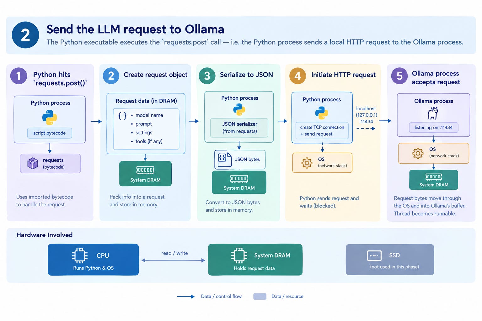
TL;DR: The Python executable executes the requests.post call - i.e. the Python process sends a local HTTP request to the Ollama process.
Hardware Involved: CPU, System DRAM
The Python process starts executing our script like any other Python script, and quickly runs into the Ollama request:
r = requests.post(
        "http://localhost:11434/api/generate",
    json={
        "model": "qwen3:8b",
        "prompt": "What's more important for Agentic AI - CPU, or GPU?",
        "stream": False,
    },
)
Unlike other Python commands, which are fully executed within the Python process, this HTTP request needs the involvement of the OS, as we will see in the steps below.
Step 1: The Python process encounters a call to the imported bytecode
In the compiled bytecode of our agentic workflow, the requests.post() call redirects the Python process towards the bytecode that was imported in Phase 1. This is needed because our script’s bytecode does not know how to execute this command. (Note that we are still within the Python process - we are just reading a different bytecode.)
Step 2: Python process creates a request object
Using the imported bytecode, the Python process creates an HTTP request with the following information:
Model name
Input prompt
Request settings (streaming, local/online request, etc.)
Information about the tools if applicable
Essentially, the Python process packages all the information that Ollama might need to run the LLM inference into a single request. This request, typically represented as a Python dictionary, is then stored in System DRAM.
Step 3: Python process serializes the request object to JSON bytes
Although the information needed by Ollama is ready in Step 2, Python objects can’t be sent directly in an HTTP request through a TCP socket. So the Python process:
Reads the Python objects (saved in step 2) from the System DRAM
Serializes them using the JSON serializer (also part of the requests bytecode.)
The output is a sequence of UTF-8 bytes which is stored back in the System DRAM.
Step 4: Python process initiates an HTTP request to the Ollama process
Now that the data needed for the HTTP request is ready, the Python process constructs the request in this step. Essentially, Python tells the OS to create a TCP connection to:
IP Address: 127.0.0.1 (localhost corresponds to this address.)
TCP Port: 11434 (this is the default Ollama listening port)
The OS establishes the TCP connection through the local loopback interface. (It does not actually leave the computer.) Once connected:
The Python process requests the OS to send the HTTP request with the JSON bytes from the System DRAM. (Stored there in step 3.)
Once complete, the Python Thread that was executing everything so far moves into a blocked/waiting state.
This is a key milestone in the CPU execution. Watch out for when this thread is reactivated. (Spoiler alert: It’s not very soon.)
Once the shoes are packed in the boxes, they are stored and ready to be picked up. The shoe manufacturer gets in touch with the shipping company to arrange for their shoes to be shipped from their factory to its destination. You can think of the Ollama process as the shipping company. Once the shipping company picks up the boxes, the shoe manufacturer just needs to wait for the delivery.
Step 5: The Ollama process accepts and parses the request
While I didn’t explicitly mention this so far, Ollama is typically already running as a separate process. (Usually started at boot, or manually with the ollama serve shell command.) The process has a thread that is in the waiting state, and is listening on its default port 11434 - the same port that Python asked to send the LLM inference request.
Note that the Ollama thread is still a CPU thread - we have not started the GPU execution just yet.
Although the shipping company’s main task is ocean shipping, they still need Trucks (CPU) to move goods to and from the container ship.
The OS executes the HTTP transfer requested in step 4 on the TCP port by:
Moving the request bytes from the Python process into the local socket/network stack
Placing the bytes into Ollama’s socket receive buffer
Marking the Ollama thread as runnable
The OS then schedules the now ready Ollama thread on an available CPU core. The handshake between the two processes has completed, and the execution will now be taken forward by the Ollama process.
At the end of Phase 2:
The Python process has handed off information for LLM inference to the Ollama process.
Before we continue: What would inference on a cloud model look like?
Subscribe for free to see this section:
Phase 3: Ollama prepares the GPU for LLM inference
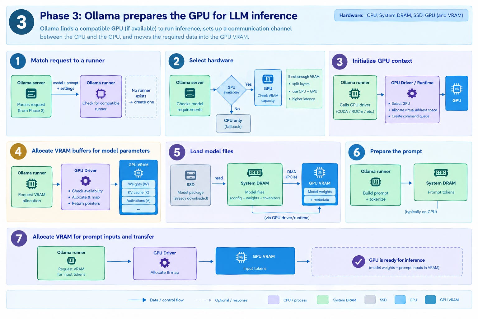
TL;DR: Ollama finds a compatible GPU (if available) to run inference, sets up a communication channel between the CPU and the GPU, and moves the required data into the GPU VRAM.
Hardware Involved: CPU, System DRAM, SSD and GPU (and it’s VRAM)
At the end of Phase 2, the Ollama process has received the LLM inference request from the Python process. Now, it’s time to start the LLM inference. But since LLM inference will be running on a GPU, the Ollama process still has some preparation left to do.
Before going into the steps, let me define two key terms used in the context of Ollama execution:
Ollama server: The dispatcher/scheduler that listens to the TCP port, parses LLM inference requests, and routes work to the Ollama runner.
Ollama runner: It is a model-specific execution setup - it contains the model’s architecture metadata, inference backend configuration, pointer to loaded model weights, GPU/CPU memory allocations, KV-cache management, and workspace buffers. Basically, it is a reusable environment for inference using a specific LLM model.
Everything we have seen so far has only involved the Ollama server and its process. Depending on the Ollama version, backend and platform, a runner may be represented by a separate process/threads.
If anyone reading this knows more about how threads are scheduled between the server/runner, I’d love to hear more in the comments.
In our shipping example, you can think of Ollama server as the entity that manages road operations, while Ollama runner is the entity that manages operations within the port. The former is usually more flexible and can handle different tasks. However, the latter could depend on the specific ship type, loading requirements, etc. In this phase, both entities work together to start loading the ship efficiently.
Step 1: The Ollama server matches the request to a runner
The Ollama server parses the HTTP request, reads the JSON bytes, and recreates the model name, prompts, tool schemas and other settings needed for LLM inference. Then, the Ollama server looks at the model name and checks whether it already has a compatible runner.
If a compatible runner is available, Ollama reuses it.
If no runner exists, Ollama must create one.
Since this is the first (and only) LLM inference request, let’s assume the runner does not exist and walk through all the steps.
Step 2: Ollama selects the hardware for LLM inference
The Ollama server examines the hardware and model requirements and decides where the inference can run. If there is no compatible GPU, the LLM inference runs directly on the CPU. While this is not impossible for some small models, this won’t be the focus of this post.
If the system has a compatible GPU, the Ollama server compares the available GPU VRAM space with the memory requirement for the LLM model that’s requested. Ollama estimates the memory required for inference based on the model, context/KV-cache requirements, GPU configuration, and other runtime allocations.
If Ollama determines that the GPU VRAM does not have enough space, then a hybrid CPU/GPU inference path is taken:
GPU VRAM accommodates data for some of the LLM layers
Data for the other layers is kept in the System DRAM
Some model layers execute on the GPU while others execute on the CPU, with intermediate data transferred between the CPU and GPU
Hybrid inference is a very interesting problem, but the CPU-GPU transfers can add significant latency and energy overhead. Ideally, we want to run models that fit completely in GPU VRAM - which is what we will assume for the rest of this post.
Say our shipping destination is accessible by road, train, flight, or ships, then the shipping company can find the best fit depending on the load to be shipped.
Step 3: The Ollama runner initializes a GPU execution context
To use the GPU for inference, the Ollama runner asks the GPU runtime (CUDA, ROCm, Metal, etc.) to make a driver call to create the GPU context for the upcoming inference. This means the GPU driver:
Allows Ollama to use one of the available GPUs
Allocates GPU virtual address space to Ollama and maps it to physical VRAM locations
Creates a command stream/queue between the CPU (Ollama runner process) and the GPU
Essentially, Ollama can now access the GPU via its driver.
Step 4: The Ollama runner allocates GPU VRAM buffers for model parameters
Once the CPU-GPU communication channel is set up, the Ollama runner informs the GPU about the VRAM allocation for the inference. (This, like any CPU-GPU request, happens via the GPU runtime and driver - I won’t explicitly mention this going forward for brevity.) This request looks like this:
Allocate W bytes for GPU-resident weights
Allocate K bytes for KV cache
Allocate A bytes for activations
…
The driver looks at this request, checks available VRAM, allocates space, maps it to virtual addresses, and returns the information to the Ollama runner.
The GPU Driver and runtime represent the container ship crew - the shipping company needs to check with them before loading anything on the ship.
Step 5: The Ollama runner reads the local model files
Before this step, it is assumed that the required LLM model is already downloaded onto your SSD using the ollama pull command. This model package includes the model configuration (the number of layers, how they are connected, quantization, etc.), model weights, and also the data that will be used by the tokenizer.
Before Ollama can start inference:
It fetches the model package data from the SSD into the System DRAM.
Once the data is in the RAM, the Ollama runner submits a data transfer request to the GPU.
The GPU Direct Memory Access (DMA) engine moves the data into the VRAM spaces allocated earlier, typically through a PCIe interface.
For the conventional discrete-GPU host-to-device path, even when inference is fully done on the GPU, any data stored in the SSD needs to pass through the System DRAM. This becomes a major bottleneck if the model weights, KV cache, and other inference states cannot be fully stored in GPU VRAM. Datacenter architectures increasingly use specialized data-movement and infrastructure processors to reduce CPU overhead and improve data movement, such as Nvidia’s Bluefield DPU.
Moving goods from one mode of transport to another is also a time-consuming task in ports. There are some very creative solutions deployed to speed this up. For example, a log barge (ship that carries wooden logs) simply dumps its entire load onto the water, which allows it to quickly continue to its next assignment. Ore ships also have special docks which are directly connected to train tracks to speed up the unloading process.
Step 6: The Ollama runner prepares the prompt
So far, Ollama was focused on preparing the model for inference. Now it’s time to shift focus to the prompt. Before the GPU can run inference, Ollama must turn the structured chat request into a model-specific prompt representation. This means two things:
Use the model’s chat template to define how roles (system/user) and tools are represented for the model being used.
Convert the prompt string into tokens. (This step is called tokenization.)
After tokenization, the prompt is stored in the System DRAM, waiting to be made visible to the GPU.
I’m skipping the specifics of this step as it varies based on the models. But it’s noteworthy that these computations are typically handled on the CPU rather than the GPU in systems like this. Although it is small relative to the actual inference, it becomes non-trivial for very large prompts, or in a system handling multiple parallel agentic requests.
Step 7: The Ollama runner allocates GPU VRAM buffers for prompt inputs and makes the transfer
Much like what was done with the model package data, the Ollama runner also requests VRAM space for the input tokens and receives pointers to the virtual address space.
Once the required model state and input data are available to the GPU, the GPU has the data needed to start inference.
Typically, the input size is much smaller than the model size, and is also short-lived. (Although a large context/tool result can make prompt input and KV cache significant.)
At the end of Phase 3:
Ollama has set up a communication channel with the GPU and has placed the model weights and prompt inputs in GPU VRAM.
Phase 4: GPU executes the LLM inference
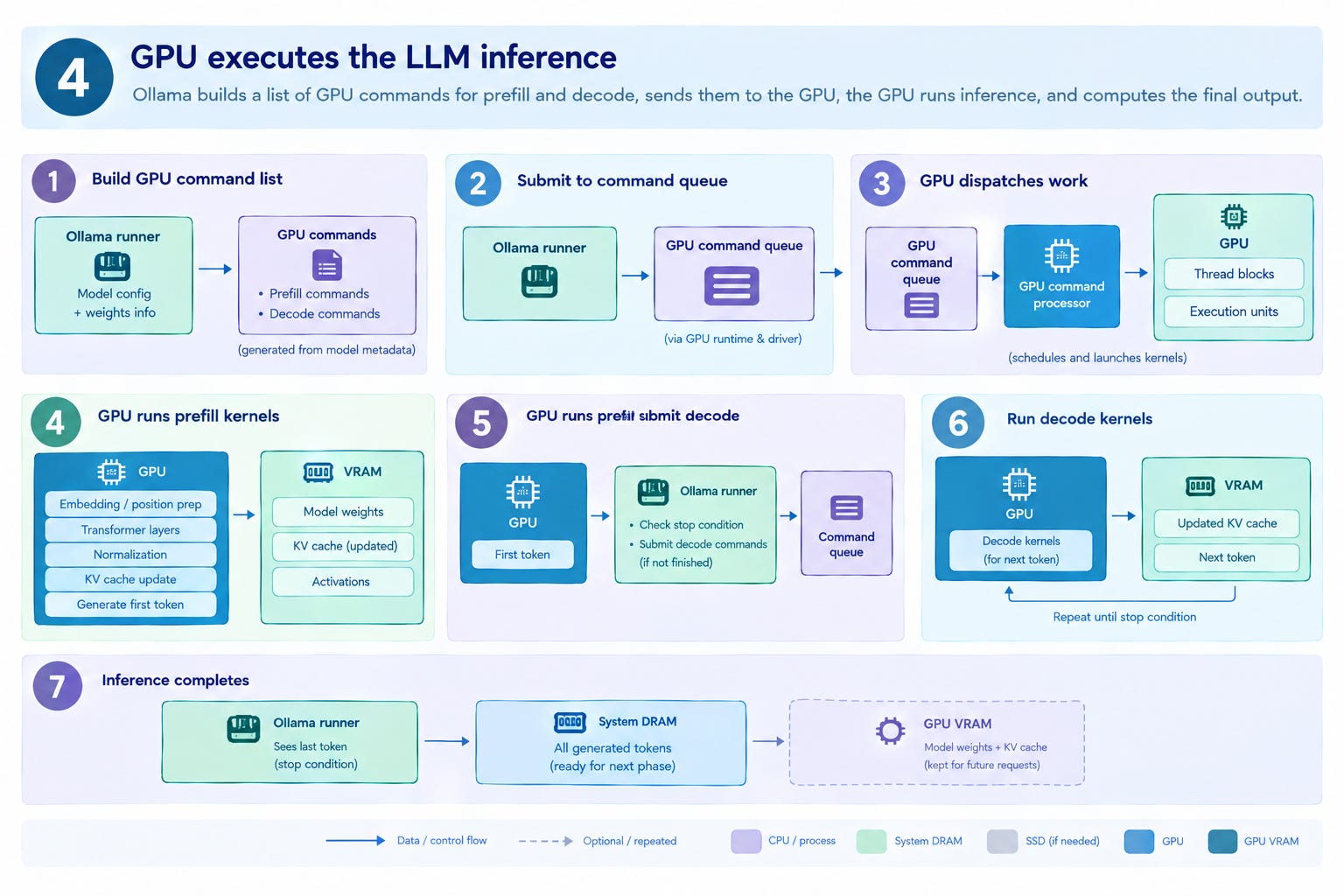
TL;DR: Ollama builds a list of GPU commands for prefill and decode, sends them to the GPU, the GPU runs inference, and computes the final output.
Hardware Involved: CPU, System DRAM, (SSD if needed), and GPU (and it’s VRAM)
We’re finally at the long-awaited inference stage. (Longer than I expected too, to be honest.)
Since this post is focused more on the interaction between the CPU and GPU, I won’t be going into all the details of LLMs. There is a lot of content that already talks about this, and I might write a dedicated post myself if I feel I have something unique to add.
For this post, we will be looking more generally at how (and how many times) the CPU sends work to the GPU. At a high level, (autoregressive) LLM inference is broken down into two stages:
Prefill stage: The input prompt is processed to generate the first output token
Decode stage: Additional tokens are generated one at a time. Each selected token becomes input to the next decode pass.
Another simplifying assumption in this post is that the LLM output is “non-streaming” - that means Ollama only sends the output back to the Python process at the end of the decode stage for all the tokens. With streaming outputs, there would be a lot more communication between Ollama and the Python process.
If the ship’s journey includes multiple stops, then the prefill stage, and each pass of the decode stage represent the ship’s journey from one port to the next. A streaming LLM inference call would be like having to unload a few containers at every stop.
With that said, here’s how the GPU actually runs inference.
Step 1: The Ollama runner builds a model-specific list of GPU commands
In the last phase, although Ollama was able to move the weights and input prompt into the GPU VRAM, the GPU still does not know what to do with them. The Ollama runner takes the configuration information in the model package read in the last phase to an inference engine (like llama.cpp) and comes up with an ordered list of commands. The command sequence would roughly look like this:
Prefill stage:
Run input kernel (embedding/position preparation)
Evaluate transformer layer 0
Evaluate transformer layer 1
…
Evaluate last transformer layer
Run normalization kernel
Write prompt K/V values to KV cache
Generate the first output token
Record a completion event for the prefill stage
Decode stage:
For each new token
Run input kernel (embedding/position preparation)
Evaluate transformer layer 0
Evaluate transformer layer 1
…
Evaluate last transformer layer
Run normalization kernel
Append new K/V values to KV cache
Generate the next token
At the last token, record a completion event for the decode stage
What each of these commands means does not matter for this post. I just added them to show that an inference call is broken down into multiple GPU commands, and each of them is composed of one or more kernels, each with a large number of arithmetic operations. For example, a single attention layer might include separate or fused kernels for Q/K/V handling, score computation, causal masking, softmax/reduction, and value accumulation.
Loading a ship is not always as simple as “move containers onto the ship as they arrive on the trucks.” When a large ship is being loaded, there is a specific order of operations to ensure the ship is balanced, deliveries are coordinated, and there is no chemical/combustion risk. The GPU commands for each pass are similar to the ship crew’s plan to start loading containers to the ship.
Step 2: Ollama submits Prefill commands to the GPU command queue
Ollama (through the GPU runtime and driver) submits the ordered list of commands to the GPU command queue.
The command queue is not a physical hardware entity - it is a driver abstraction that separates the command generation (by the CPU) from the command consumption (by the GPU).
Step 3: The GPU command processor dispatches work for Prefill
Once the command queue starts to get filled, the GPU command processor and scheduling hardware consume the submitted work and dispatch kernels for execution. This involves:
Dividing the work into multiple GPU thread blocks
Assigning each thread block to an available execution unit
In other words, each Ollama command (more precisely, each kernel) specifies what operations to run - but the GPU runtime and hardware execute the kernel across many parallel threads, grouped into thread blocks or equivalent execution units.
Think of the command queue like the loading area where the trucks drop off the container boxes. And the command processor is the loading arm that moves containers to different parts of the ship based on the predefined plan.
Step 4: GPU computes the Prefill kernels and produces the first token
This is the real “GPU execution”.
The massively parallel GPU threads execute the arithmetic, logic, and memory operations in the kernels and update the KV cache in the VRAM based on the input prompt. The kernel also generates the first output token.
I know that dumping this entire GPU computation in one sentence does great injustice to the advanced microarchitecture of modern GPUs - but those details are vendor specific, and beyond the scope of this post.
Step 5: Ollama reads the token and submits the decode pass
The output token is made available to the CPU/Ollama runner, which may involve transferring a small amount of data from GPU memory to host memory. The Ollama runner then checks the stop condition. (LLMs can generate a special end-of-sequence (EOS) token to indicate that generation should stop.)
If the generated token is not the last token, Ollama submits commands for the decode pass to the command queue, which is then picked up by the GPU command processor.
Step 6: GPU computes one pass of decode kernels and produces another token
The execution is very similar to steps 3 and 4 - the GPU command processor dispatches work for the decode pass, the GPU threads execute the kernels, and a new token is generated. The KV cache is updated with this new token. The token is sent back to Ollama to trigger the next decode pass. (or end the inference if the stop condition is met.)
Step 7: Ollama hits the stop condition, and the LLM inference completes
Steps 5 and 6 are repeated until the last token is generated. Once the Ollama runner sees the last token, it stops sending decode commands to the GPU command queue, and the LLM inference is officially complete. All the generated tokens are already present in the System DRAM, ready to be used in the next phase. The updated KV cache, along with the model weights can continue to remain in the GPU VRAM in case there are future inference requests. (More on that in future posts.)
Our shoe manufacturer’s destination is the stop condition for our shipping request. After reaching there, the ship journey for the shoes would have come to an end.
At the end of Phase 4:
Ollama sent commands to the GPU to complete the LLM inference. The output tokens are available in the System DRAM.
Phase 5: Ollama returns the inference response and the Python script finishes execution
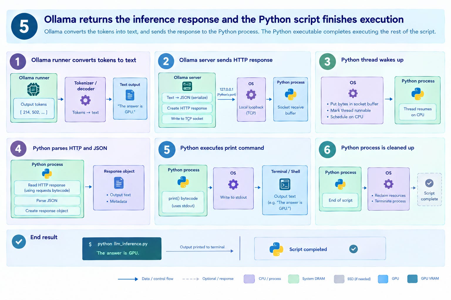
TL;DR: Ollama converts the tokens into text, and sends the response to the Python process. The Python executable completes executing the rest of the script.
Hardware Involved: CPU, System DRAM
The steps in this phase are very similar to what we saw in phases 1 and 2 - except this time, Ollama needs to send data to the Python process.
We are back on land now. The ship is unloaded, containers are moved into trucks and are driven to their final destinations.
Step 1: The Ollama runner converts output tokens into text
This is the opposite of the tokenization process that was done in Phase 4 to the input prompt. Ollama uses the tokenizer to decode the output tokens into human-readable text.
Step 2: The Ollama server process sends an HTTP response with JSON data
Ollama server converts the output text into UTF-8 bytes using the JSON serializer.
Then, Ollama creates an HTTP response with the output bytes as the response body.
Finally, Ollama writes the HTTP response to the TCP socket associated with the waiting Python process. (The IP address is still 127.0.0.1 as it is a local HTTP response. TCP port is the one allotted to the Python process by the OS.)
Step 3: The Python thread wakes up
After the Python thread sent the HTTP response to Ollama in Phase 2, it was placed in a waiting state - waiting for this very moment.
When Ollama writes the response:
The OS places the response bytes in Python’s socket receive buffer,
The OS marks the Python thread as runnable.
The OS assigns the thread to an available CPU core.
This resumes the Python process to execute the rest of the script.
The destination side entity of the shoe manufacturer is notified of the upcoming delivery.
Step 4: Python process parses HTTP and JSON
The active Python thread uses the requests bytecode to read the HTTP response, extract the JSON body, and create a response object containing Python strings and metadata.
Once this object is created, it marks the end of the original source line:
r = requests.post(...)
Step 5: The Python executable executes the print command
We are done with the LLM inference.
We are done with the Ollama request.
Now, Python executes the bytecode for the print() function, which writes to standard output. The OS writes to the destination connected to stdout, usually displaying the output text in the shell window.
Step 6: Python process is cleaned up
Once the Python executable reaches the end of the script, the OS reclaims the resources allocated to the Python process - which officially marks the end of the script.
Once the shoes are delivered to the right place, the shipping request can be marked as complete.
At the end of Phase 5:
The output from the LLM inference is printed, and the script completes execution.
Conclusion (Finally!)
Ever since ChatGPT, there has been a lot of chatter about AI hardware that gets oversimplified to sound like this:
“Run LLM inference on the GPU, everything else on the CPU”
My goal was to go one layer below this to understand exactly what the interaction between a CPU and a GPU looks like.
It took a lot of time for me to put this post together, but I needed to do this before I could meaningfully participate in the ongoing conversation about Agentic AI hardware.
I hope reading the post can help you do the same.